Multiple Linear Regression
Linear Regression is using a straight line to describe a relationship between variables. It finds the best possible fit through minimizing “error” of the model. Simple linear regression uses one independent variable and one dependent variable and multiple linear regression uses more than one independent variable with one dependent variable. Multivariate linear regression uses more than one dependent variable. I most often use multiple linear regression so I’ll discuss that here.
1. Load your packages
library(ggplot2)
library(dplyr)
library(broom)
library(ggpubr)
library(moderndive)
library(readr)
library(readxl)
library(skimr)
library(tidyverse)
2. Load the data
data = read_xls("PS206767-553247439.xls", sheet = 2)
data = data %>%
  select(1, 4, 10, 39) %>%
  mutate(height = as.numeric(`Height (cm)`),
         dose = as.numeric(`Therapeutic Dose of Warfarin`),
         gender = as.factor(Gender)) %>%
  select(1, 5:7) %>%
  filter(gender != "NA") %>%
  drop_na()
data should have appeared in your Global Environment (in the upper right side of the RStudio screen)
After you load data, always check it out to make sure you called what you meant to…I like skim or glimpse for this
skim(data) | Name | data |
| Number of rows | 4443 |
| Number of columns | 4 |
| _______________________ | |
| Column type frequency: | |
| character | 1 |
| factor | 1 |
| numeric | 2 |
| ________________________ | |
| Group variables | None |
Variable type: character
| skim_variable | n_missing | complete_rate | min | max | empty | n_unique | whitespace |
|---|---|---|---|---|---|---|---|
| PharmGKB Subject ID | 0 | 1 | 11 | 11 | 0 | 4443 | 0 |
Variable type: factor
| skim_variable | n_missing | complete_rate | ordered | n_unique | top_counts |
|---|---|---|---|---|---|
| gender | 0 | 1 | FALSE | 2 | mal: 2637, fem: 1806, NA: 0 |
Variable type: numeric
| skim_variable | n_missing | complete_rate | mean | sd | p0 | p25 | p50 | p75 | p100 | hist |
|---|---|---|---|---|---|---|---|---|---|---|
| height | 0 | 1 | 168.06 | 10.84 | 124.97 | 160.02 | 167.89 | 176.02 | 202 | ▁▂▇▆▁ |
| dose | 0 | 1 | 31.23 | 17.06 | 2.10 | 20.00 | 28.00 | 39.97 | 315 | ▇▁▁▁▁ |
glimpse(data)Rows: 4,443
Columns: 4
$ `PharmGKB Subject ID` <chr> "PA135312261", "PA135312262", "PA135312263", "P…
$ height <dbl> 193.040, 176.530, 162.560, 182.245, 167.640, 17…
$ dose <dbl> 49, 42, 53, 28, 42, 49, 42, 71, 18, 17, 97, 49,…
$ gender <fct> male, female, female, male, male, male, male, m…Check for correlation
data %>% get_correlation(dose ~ height, na.rm = T)# A tibble: 1 x 1
cor
<dbl>
1 0.315Just to get an idea of the linear relationship….there is about 30% correlation here between our outcome variable and the continous predictor, height.
3. Check your assumptions
There are a number of assumptions that need to be correct in order to properly use multiple regression.
- Independence of observations
Independence of observations means each participant is only counted as one observation. The statistical assumption of independence of observations stipulates that all participants in a sample are only counted once. This is satisfied if we’re using one observation per person.
- Normality
Use hist() to test the dependent varible for a normal distribution.
hist(data$dose)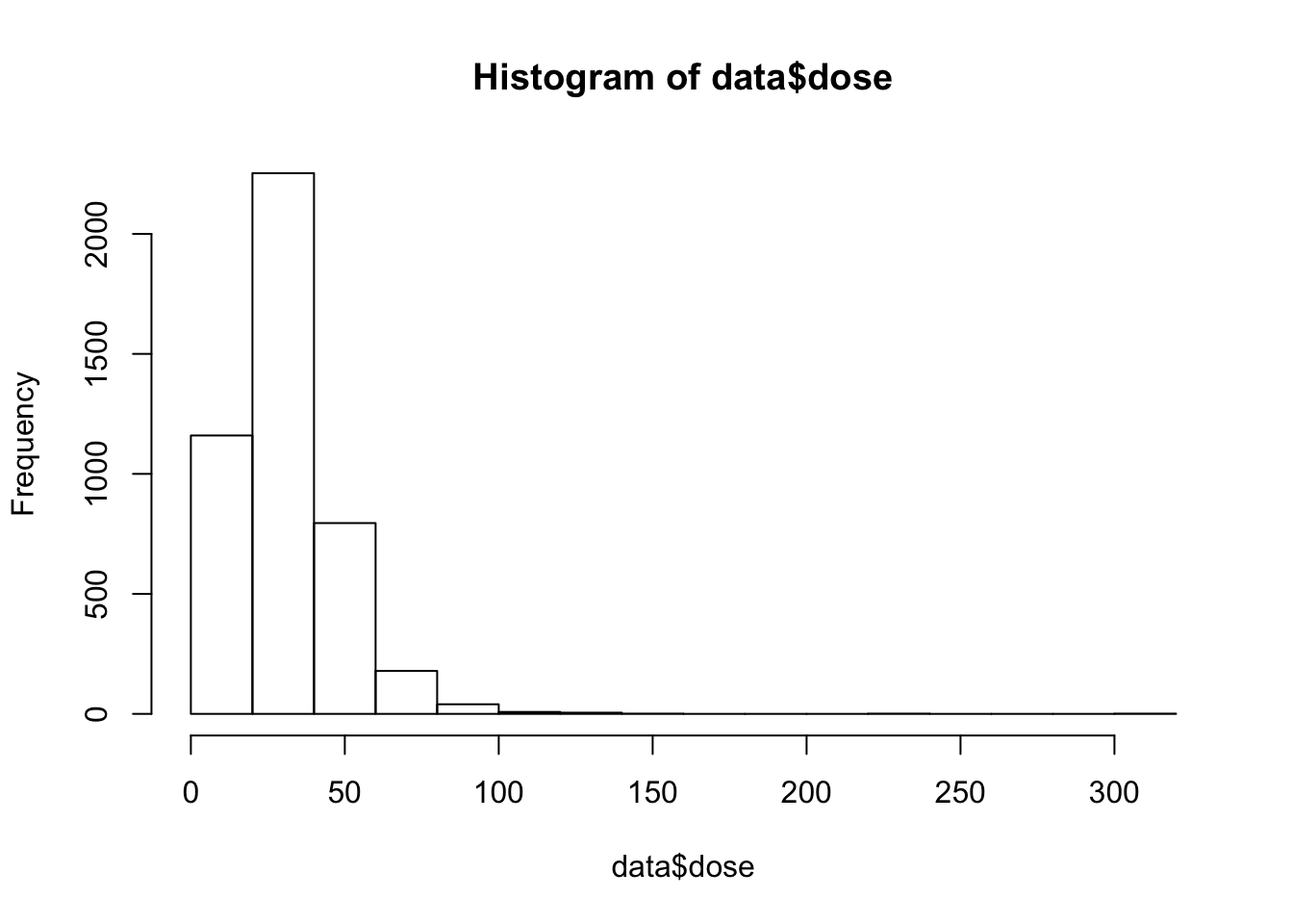
This distrubtion is a lil’ skewed and we should log transform the data.
data$outcome = log(data$dose)and re-plot…
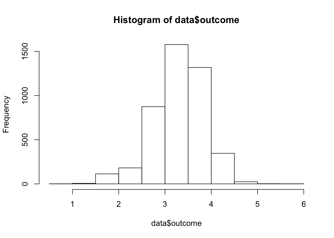
This plot is much more bell-shaped and we can move on.
- Linearity should be assessed using scatterplots of the outcome (dependent) variable with each of the included predictors (independent variables).
data %>% filter(gender != "NA") %>% ggplot(aes(outcome, height, group = gender, color = gender)) + geom_point() +
geom_parallel_slopes(se = F) +
theme_bw()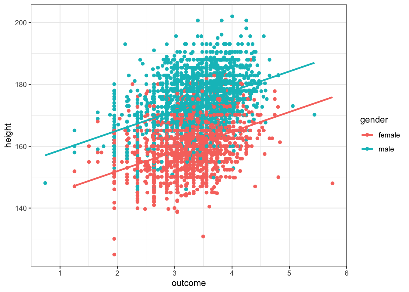 In this plot we’ve visualized both the numeric predictor variable, height, and the factor predictor, gender, by setting the aesthetics for each of these variables.
- Homoscedasticity The fourth assumption is equal variance among the residuals…which we will test after running the model by plotting residuals.
4. Run the model
Linear regression syntax is super straighforward in R. The model is given as outcome ~ predictor + predictor and you can call it with the lm() function. I’ve included the wrapper summary() so we can get the statistics back from the regression. Alternatively, use the moderndive package and get_regression_table() to get the same output.
fit = lm(data = data, outcome ~ gender + height)
summary(fit)
Call:
lm(formula = outcome ~ gender + height, data = data)

Residuals:
     Min       1Q   Median       3Q      Max
-1.95202 -0.28410  0.03265  0.32105  2.78849

Coefficients:
              Estimate Std. Error t value Pr(>|t|)
(Intercept) -0.7451039  0.1385046   -5.38 7.85e-08 ***
gendermale  -0.2720412  0.0190291  -14.30  < 2e-16 ***
height       0.0250611  0.0008626   29.05  < 2e-16 ***
---
Signif. codes:  0 '***' 0.001 '**' 0.01 '*' 0.05 '.' 0.1 ' ' 1

Residual standard error: 0.4912 on 4440 degrees of freedom
Multiple R-squared:  0.163, Adjusted R-squared:  0.1626
F-statistic: 432.3 on 2 and 4440 DF,  p-value: < 2.2e-16
or use moderndive…
get_regression_table(fit)# A tibble: 3 x 7
term estimate std_error statistic p_value lower_ci upper_ci
<chr> <dbl> <dbl> <dbl> <dbl> <dbl> <dbl>
1 intercept -0.745 0.139 -5.38 0 -1.02 -0.474
2 gendermale -0.272 0.019 -14.3 0 -0.309 -0.235
3 height 0.025 0.001 29.1 0 0.023 0.0275. Plot Residuals
Super important to come back and check homoscedasticity (equal variance) of the residuals. Do this by plotting the same lm() used previously. Residuals are calculated from model error and you can think about them as unexplained variance.
par(mfrow = c(2,2)) ## show 4 plots at once
plot(fit) ## plot residuals
What you want here is, basically, horizontal lines centered around 0 for each of the plots except the Q-Q plot which should follow along the theoretical quantiles.
data$predicted <- predict(fit)   # Save the predicted values
data$residuals <- residuals(fit) # Save the residual values

# Quick look at the actual, predicted, and residual values

data %>% select(outcome, predicted, residuals) %>% head()
# A tibble: 6 x 3
outcome predicted residuals
<dbl> <dbl> <dbl>
1 3.89 3.82 0.0712
2 3.74 3.68 0.0587
3 3.97 3.33 0.641
4 3.33 3.55 -0.218
5 3.74 3.18 0.554
6 3.89 3.44 0.453 Here’s another, much prettier plot of residuals.
data %>%
  sample_frac(.5) %>%
  gather(key = "gender", value = "x", -outcome, -predicted, -`PharmGKB Subject ID`, -residuals, -dose, -height) %>%  # Get data into shape
  ggplot(aes(x = height, y = outcome)) +
  geom_segment(aes(xend = height, yend = predicted), alpha = .2) +
  geom_point(aes(color = residuals)) +
  scale_color_gradient2(low = "blue", mid = "white", high = "red") +
  guides(color = FALSE) +
  geom_point(aes(y = predicted), color = "gray", alpha = .5) +
  facet_grid(~ x, scales = "free_x") +  # Split panels here by `iv`
  theme_gray()
That’s really the basics of performing a linear regression in R.
Heidi E. Steiner
Senior Clinical Data Scientist
I love coding in R, biostatistics, and reproducible clinical research.